This week’s exercises
| Section | Exercise | Importance | Time |
|---|---|---|---|
| 0.0 | einops operations & broadcasting | 3/5 | 45 min |
| 0.0 | einsum | 4/5 | 15 min |
| 0.2 | ReLU | 3/5 | 5 min |
| 0.2 | Linear | 4/5 | 10 min |
| 0.2 | Simple MLP | 4/5 | 15 min |
| 0.2 | Training loop (read) and validation loop | 5/5 | 30 min |
| 0.2 | Conv2d | 3/5 | 15 min |
| 0.2 | BatchNorm2d | 3/5 | 20 min |
| 0.2 | AveragePool | 2/5 | 5 min |
| 0.2 | ResidualBlock | 4/5 | 25 min |
| 0.2 | BlockGroup | 4/5 | 12 min |
| 0.2 | ResNet34 | 4/5 | 35 min |
| 0.2 | Verify your model’s predictions | 3/5 | 10 min |
| 0.2 | Aside: hooks (read) | — | 10 min |
| 0.3 | opt_fn_with_sgd | 4/5 | 15 min |
| 0.3 | Adam | 3/5 | 20 min |
| 0.4 | log_back | 3/5 | 8 min |
| 0.4 | unbroadcast | 3/5 | 15 min |
| 0.4 | multiply_back0 and multiply_back1 | 2/5 | 12 min |
| 0.4 | forward_and_back | 4/5 | 15 min |
As you work through these exercises (and in general going forward), if you find yourself stuck or spending way more time on an exercise than the estimate, have someone in your group peek at the answer or prompt an LLM for hints. No single exercise is worth laboring over too too much.
Tensors, Einops, and Einsum
This section is going to be super brief, and I’m not really going to explicitly walk through any of this. Instead, as is kind of the theme of this entire program, I think it’s best to just learn by doing.
What’s a Tensor? is an OG video from physicist/professor Dan Fleisch and can help you build some stronger intuitions around what they are and how they work. Tensors are the fundamental building block of all neural networks, so it’s important that we get comfortable with them. One caveat: the video explains tensors as physicists use them, defined by how they change between coordinate systems. In ML, the word is looser. I’m no mathematician, but I basically just think of tensors as higher-dimensional matrices (n-dimensional arrays of numbers). Basically, they’re just these arrangements of numbers that either represent information itself or how to manipulate information that’s passing through the network.
Einops and einsum are these awesome notations for writing tensor operations (reshaping, reducing, multiplying) by naming each axis. It can be kind of counterintuitive at first, but then, after repeated work with them, they can become really intuitive. With good naming practices, it can make it both way faster/easier to write the code out and for someone else to read and understand it.
I’d highly recommend really sitting with all of these materials and putting effort into the explicit einops practice problems. The intuitions with it will then really solidify through section 1.1 when we actually build transformers.
Backpropagation
I’m assuming a basic level of background knowledge, but here’s a toy refresher on backprop.
Backprop is the process by which the network actually comes to do anything useful. It’s the information on which the optimizer then decides how to actually update the parameters. On a super high level, we’re calculating how bad the model’s prediction was for a task and how we should tweak each of the parameters so that its prediction is a little bit better next time.
So what is backpropagation, really? Fundamentally, it’s taking the partial derivative of the loss function with respect to every single weight and bias in the network, i.e. figuring out how much tweaking a given parameter contributes to how bad our prediction was. You can imagine how many calculations this consists of in a modern-day LLM…
But, as we know from multivariable calculus, we can take advantage of the chain rule and re-use many of the common upstream partial derivatives. For instance, say we have a simple multi-layer perceptron (MLP):
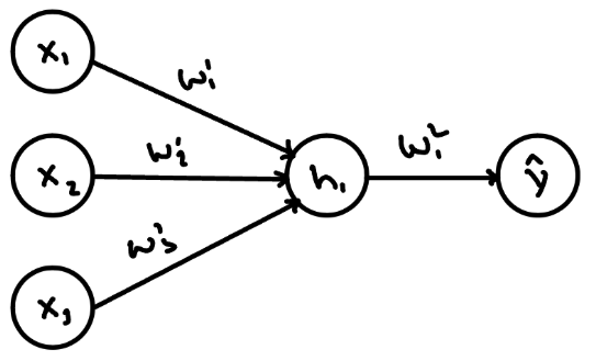
Where
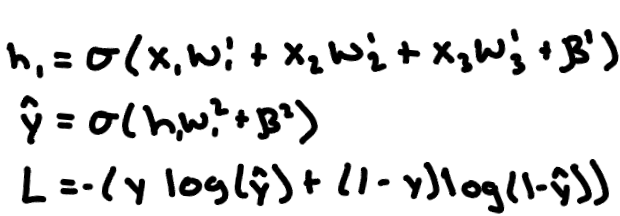
In this network, we need to find the partial derivative with respect to each of the four weights and two biases. PyTorch does this by building a computational graph to keep track of all of the network’s trainable parameters and the route by which we get from them to the loss function:
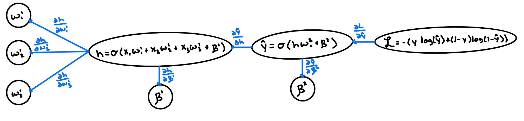
Here, we can observe that many edges are used for multiple paths from the loss function to a given parameter. Instead of recalculating each time we traverse the graph, we store these local partial derivatives for reuse. With the chain rule, the partials with respect to each of the first layer’s weights depend on the partial with respect to the node in the hidden layer.
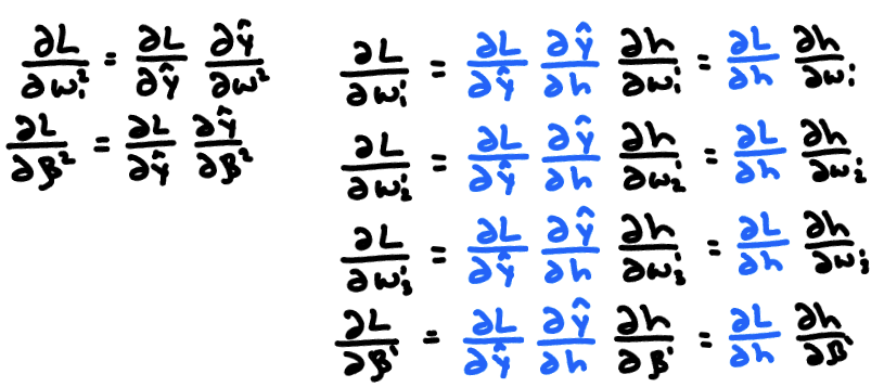
This is somewhat trivial in this example, but you can imagine how in a deep neural network, this can massively reduce the number of calculations, so long as we are careful and smart about tracking everything. One note: I’m ignoring some of the nuances that come with the shape of the tensors/matrices in each layer, but that’s somewhat beside the point.
Luckily, some great engineers have basically automated this entire process for us, and we’ll basically never have to worry about this in practice. It is, however, important to make sure we still understand the underlying mechanism.
The few 0.4 exercises for this week are just building out some of the backpropagation infrastructure/algorithms by hand. If you’ve built something like micrograd or are generally comfortable with backpropagation, feel free to skip these exercises. I will say, though, that while my above example might make backprop seem pretty simple, it can get messy sometimes with these multi-dimensional tensors, broadcasting, and topological nuances. Again, it’s not something we’ll have to be all too conscious of day-to-day, but I think these can still be a good exercise for anyone to just keep building your conceptual and abstract reasoning abilities and general comfort with everything.
Optimization
Optimizers then tell us how we actually want to update the weights based on the information gathered from the backpropagation process. All of a model’s behavior is learned through this optimization process, so understanding the dynamics of this process is critical for safety. Optimizing an imperfect objective, and the particular solution the optimizer lands on, are behind phenomena like specification gaming, goal misgeneralization, sycophancy, and even things like emergent misalignment.
Basically every optimizer and every part of training is using some form of gradient descent:
Plain gradient descent has some issues, though, such as:
- It can be prohibitively expensive (a full forward and backward pass over the entire training set for every single step)
- It can get stuck in non-optimal local minima, saddle points, or plateaus
- Alternatively, it can perpetually bounce around one of these and never settle
- It can be unstable: a step that is too large can make the loss blow up instead of going down
- Its update steps can be too large or too small depending on where in training it is and what parameters it’s updating
- Nothing in it prefers solutions that generalize, so it can overfit to the training data
Below, we’ll walk through some common alternative optimization algorithms that sought to address these issues.
Mini-batch stochastic gradient descent estimates the gradient on a random batch of examples, making each update step much cheaper and faster. This process brings in noise, but this noise is actually useful because it can help the optimizer escape local minima, saddle points, and plateaus.
Momentum then kind of brings this to the next level. The idea here is to keep a running velocity of the past gradients and integrate this into the update calculation. It’s almost literally like momentum in physics. It keeps it going in the direction it was already going. It carries the optimizer across small bumps or flat regions of the loss landscape, prevents it from getting too sidetracked by really steep gradients that are off-course, and takes it down a smoother, typically faster path towards the minima.
Adaptive step sizes (AdaGrad, RMSprop) divide each parameter’s step by the size of its recent gradients, that way ones with large or noisy gradients take smaller steps and those with small gradients take larger ones. The equation below is RMSprop; AdaGrad sums all past squared gradients instead of keeping a moving average, so its steps keep shrinking over time.
Adam combines the idea of momentum and adaptive step sizes into a single optimization algorithm.
(The math here isn’t super important, just focus on the concepts)
Adam can already use weight decay, but it adds the decay to the gradient, where the adaptive scaling weakens it for parameters with large gradients. AdamW instead seeks to learn more generalizable weights by applying weight decay directly to the weights, shrinking them towards zero to prevent overfitting and prefer simpler solutions where possible. AdamW is the default optimizer used with most transformer architectures.
We might also choose to “clip” gradients above a predetermined limit (usually by scaling the whole gradient down when its norm is too large) to stop a single bad or non-representative batch from influencing too much. We’ll also use normalization techniques like BatchNorm or LayerNorm, but we’ll get into BatchNorm in the ResNet section below.
There are also a number of hyperparameters we’ll need to “tune,” each of which can have massive effects on our training. The learning rate is a particularly important one. Too high a learning rate and our loss will never converge, too low and learning can stall (or just take a long ass time). We’ll often first warmup our learning rate by starting it near 0 and raising it linearly over the first steps of training (often the first 1–5%). We do this because our weights are initialized randomly and full-sized steps can be destabilizing. We’ll also often use a learning rate scheduler to dynamically change the learning rate over the course of training to take large steps early on during training to make fast progress and incrementally smaller steps over time to help the optimizer settle into a nice minimum.
Convolutional Neural Networks
It’s often easiest to start with CNNs for image recognition, and here, we’ll start with a small black and white 9x9 pixel image.
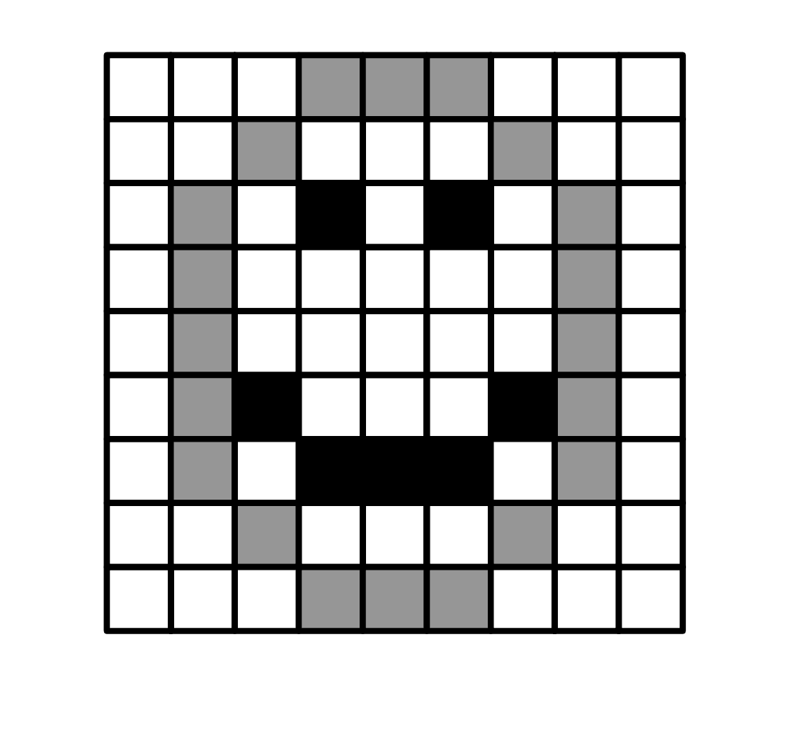
Computationally, we know each pixel of the image is represented by a number representing the intensity of the pixel along the black-white gradient (here 0 = white, 1 = gray, 3 = black). So, to the computer, it looks something more like:
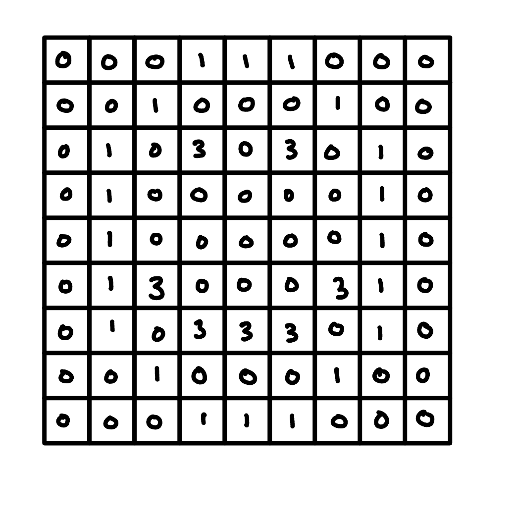
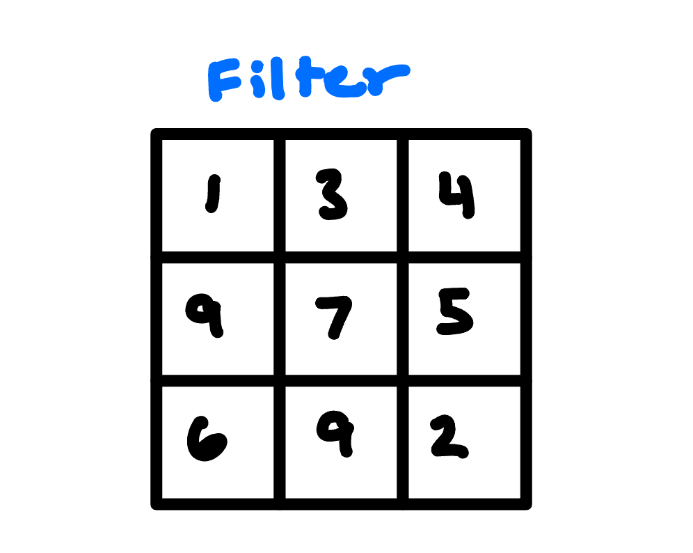
We’re assuming here, as in the picture, that there are only 3 different levels of color intensity. We then have something called a filter (also known as a kernel) which is a small grid of weights (parameters). Let’s say here that our filter is 3x3 and it is initialized randomly, like any other weights in a neural network. (Real filter weights are small numbers, both positive and negative; we use whole numbers here to keep the arithmetic easy.)
A convolution then is this mathematical process in which we slide our filter over “patches” of our original image, in this case 3x3 pixels at a time. The output is the sum-product of the filter weights and the patch values.
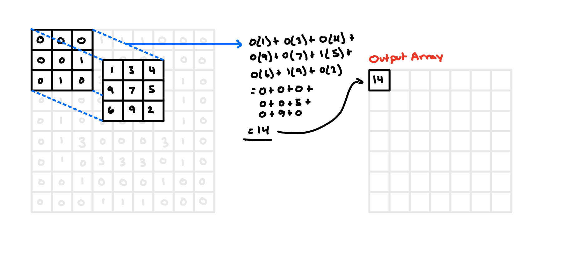
We’ll then do this for each patch of our input image, resulting in a 7x7 output array for this convolutional layer (with a stride of 1 and no padding). Notice here that the output layer is of a lower dimensionality than the input layer (just 49 numbers versus the original 81).
Two ideas make this work. Locality: each output looks only at a small patch of nearby pixels, which builds in the assumption that nearby pixels belong together. Weight sharing: the same filter slides over every position, so a filter that learns to detect, say, an edge can find it anywhere in the image, with far fewer weights than a fully connected layer.
It can get a bit more complex with more input channels (like with color images in RGB) and more convolutional layers, but we’ll skip that for this. The important point to take away from CNNs is that it is a way that a neural network is able to process a given piece of information along with its surrounding context. CNNs are included here for two reasons. First, ResNets (below) are CNNs, and they introduced the residual connections that become the transformer’s residual stream. Second, much of mech interp’s vocabulary (features, circuits) comes from early work interpreting vision CNNs (Zoom In). One contrast to keep in mind for next week: a convolution mixes a fixed local window with the same weights everywhere, while attention mixes all positions with weights that depend on the input.
Some quick definitions of CNN concepts:
- Kernel size: refers to both the size of the filter/kernel and the size of a patch
- Stride: how far the kernel moves each step. Sometimes, we’ll want to slide more than just 1 pixel over.
- Padding: adding zeros around the edges of the input. This is mostly used to control the output size (for example, keep it the same as the input), and it also lets edge pixels be covered as often as center ones.
- Channels: the number of values per pixel. Our black-and-white image has 1 input channel. An RGB image has 3: each pixel has 3 separate numbers (e.g. 224, 196, 181) for its intensity along the red, green, and blue spectrums, and each of these sits on its own 9x9 array. A filter always covers every input channel at once: for RGB, a 3x3 filter is really 3x3x3, and it adds everything up into one output number. Using several filters gives several output channels, one per filter, each detecting a different pattern.
- Pooling: a common downsampling technique in CNNs used to reduce the spatial size (height and width) while keeping the most relevant information (max pooling, average pooling, global average pooling). Pooling has no weights, and it also makes the model a bit less sensitive to small shifts in the image, which helps it generalize.
Residual Networks
In theory, a deeper network just simply has far more representational power than a shallow network. But deep networks used to be super susceptible to exploding and vanishing gradients. Better initialization and normalization (see BatchNorm below) mostly fixed that, but the ResNet authors found a second problem, the degradation problem: past a certain depth, adding layers made even the training error worse. Deep plain networks were just hard to optimize, partly because they put the input data through so many transformations that information can easily get lost or become unrecognizable along the way.
The fix to this was to add residual (or skip) connections. In a simple feed-forward network, a given layer operates only on the outputs of the previous layer. Skip connections instead add back in information from an earlier position into the input fed to our layer.
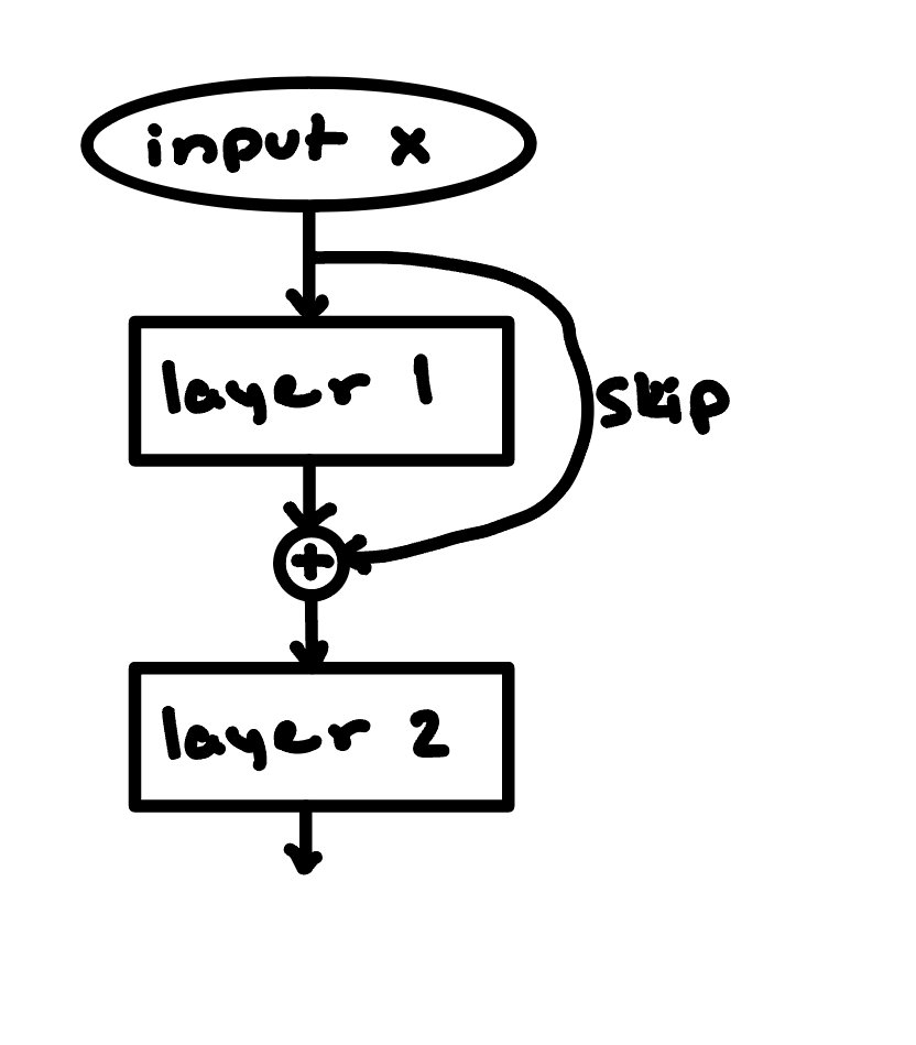
If a layer isn’t useful, it can learn to output roughly zero and just pass its input through. This has the effect of making training much more stable, preventing vanishing/exploding gradients, and making deep networks real good. Skip connections are the direct ancestor of the residual stream, one of the most important aspects of the transformer architecture and our main object of study in much of Chapter 1 (and mechinterp in general).
BatchNorm. ResNets also put a batch normalization layer after each convolution. For each channel, it normalizes the activations to mean 0 and variance 1 across the batch (and across height and width), then applies a learned scale and shift. In training mode, it uses the current batch’s statistics and updates a running average of them. In eval mode, it uses the running average instead. So always call model.eval() before using a trained model, or its outputs will depend on whatever else is in the batch.